
This post is a continuation of last weekend’s “Seeking Linearity – Part 1“, where we investigate reducing the noise from trading models.
To start off, I’m making a small alteration to the described formula to sharpen it up by normalizing for long-term volatility, as follows:
- A = Average_Price(Days) – Average_Price(Weeks)
- B = A/ Last_Price
- C = B/ Standard_Deviation(B, Years)
- D = Percent_Rank(C, Years)
The simple, frictionless equity curve trading the SPY according to the very same rules from our last post, looks like this:
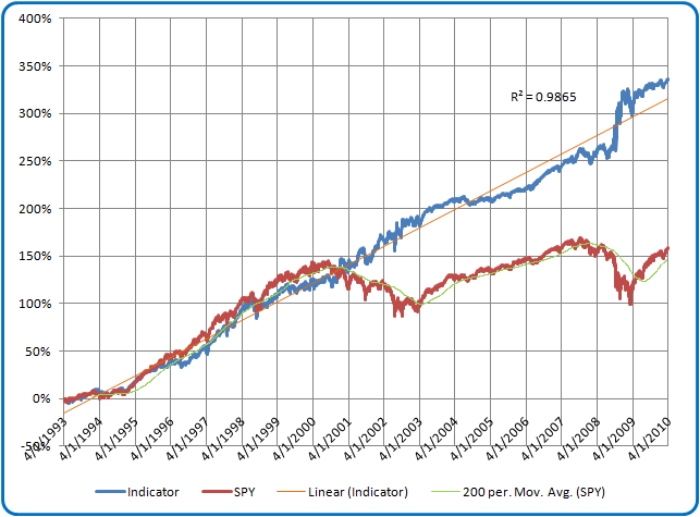
As shown, the simple indicator does a fairly good job in its own right at self-attenuation. Let’s take a moment to consider what attributes allow it to do so:
- Daily Return Smoothing/ Noise Reduction
- [Fixed] Cycle Consideration
- Volatility Normalization
- Real World Distribution Factoring
- [Binary] Environmental Rule Shifting
That last point is my least favorite aspect. We’ll take a look at that and Adaptive Cycle improvements in later iterations. Then we will focus on the original premise of this series, which is using the raw equity curve as a feedback element in its own right. In fact, since the base indicator does a fairly good job of that on its own, here is a first look at the concept, applying our little indicator to its very own equity curve (albeit using more liberal buy-sell rules). The derivative equity curve results for this approach are shown below:
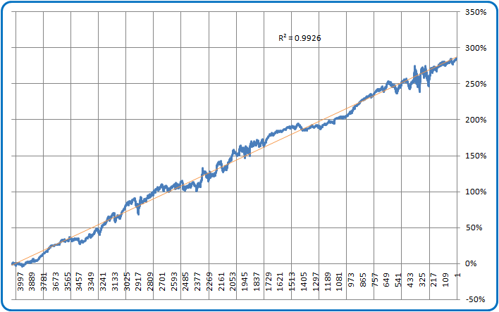
Well, not too bad as a second attenuation attempt. However, beyond the long-term linearity, the feedback loops created around the line of best fit are pretty outrageous! Perhaps a more nuanced gradient-based or other approach will do a better job of managing that noise.